Rendering the satellite image
How Dayside turns a heightfield and a climate map into a satellite image, and how to steer the result without guessing.
Colour in Dayside is computed from the ground itself. A render reads the section's signed heightmap and its Köppen climate crop, works out where water flows, where snow survives the summer and what material each patch of ground is made of, then composites all of it at the section's own pixel size. You start the render by hand, watch it arrive at three resolutions, and adjust.
Starting a render#
Put the top bar in Render mode. Acquire is the primary button, both at the right of the top bar and pinned to the bottom of the Controls panel. Its label always states the state: Acquire on a section with no frame, Queued while it waits, Acquiring N% while it runs, and Re-render once the frame has gone stale or a pass failed.
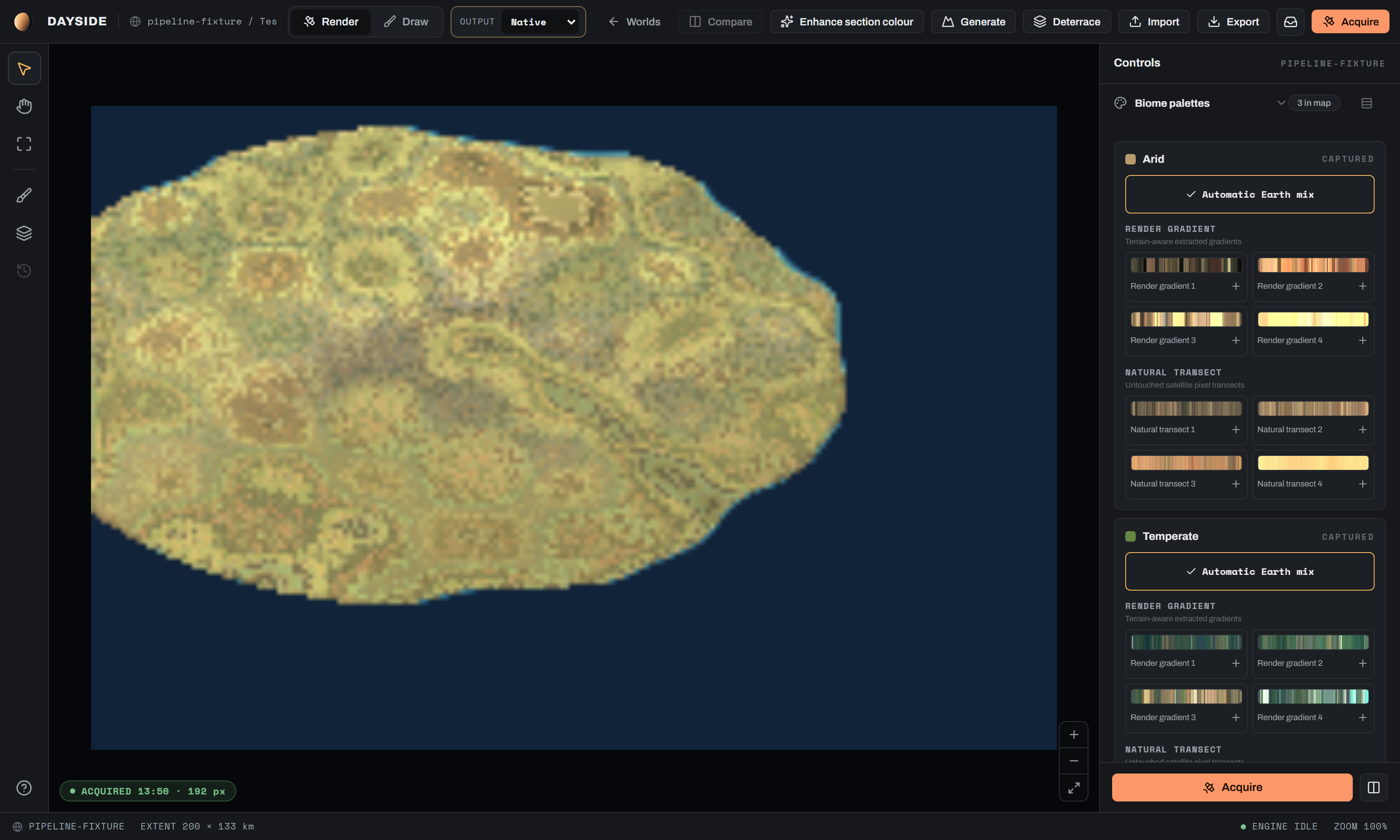
A render never fires by itself. The one exception is terrain synthesis: when Generate finishes, the editor reloads the section and starts a colour render for you, because the heightmap under the old frame no longer exists.
Queue, priority and cancel#
One render runs per world at a time. While a render is queued the canvas shows QUEUED, POSITION n · <PRIORITY> PRIORITY and offers Prioritise and Cancel. While it runs you get ACQUIRING · N% with a PASS and RESOLUTION n px readout.
Cancellation is cooperative. The flag is checked between passes and at every stage boundary, and a cancelled render keeps everything it already finished. The canvas holds the last frame it published and drops back to PREVIEW STALE.
It is CPU work#
The colour render uses no GPU. Flow routing runs on in-house numba kernels and the rest is numpy and scipy. The native composite spreads over up to four threads automatically and produces bitwise-identical output at any thread count.
Two operations in Dayside want a GPU, and this is neither of them: Generate (terrain diffusion) and Enhance section colour.
For scale: flow routing costs roughly 1.5 to 2.3 seconds on the default 4096 px analysis grid, plus a one-off JIT warmup of about 1.3 seconds that is then cached on disk. The hillshade alone is about 5 seconds at 16K and holds several GB of transient while it runs.
What the render computes, in order#
- Decode. The signed heightmap is decoded to metres through the section's own decode contract. Sea level is 0 m by definition: land positive, ocean negative.
- Flow routing. A priority-flood depression fill, then rain-weighted multi-flow accumulation. A ring of the neighbouring world canvas is spliced around the section so drainage entering from outside is approximated. This produces a catchment area in km² per cell, a depression-fill depth in metres, and the routing's own sea mask. It runs on the undownsampled heightmap.
- Analysis resample. Everything from here until the composite runs on the analysis grid, whose long side is capped by Texture detail (
analysis_long_side, default 4096 px). - Water and land. Below-sea cells the routing could not connect to open ocean are treated as enclosed pockets and become land for every stage that follows, so a deep pocket floor reads at sea-level temperature. That is the Death Valley reading. One distance transform to the ocean then serves both the seasonal climate model and the beach ring.
- Temperature. A latitude curve, a continentality shift derived from distance to the sea, and a 6.5 °C/km lapse rate. The curve needs the section's centre latitude and extent; without them the section is unlocated, takes a uniform
t_eq_c, and has no seasonal swing at all. - Data maps. Slope, multi-scale concavity and a multi-scale moisture proxy, every window given in km. Routed drainage then replaces most of the proxy wherever the terrain genuinely drains, and hands back to it inside depression fills where routed values mislead in both directions.
- Texture base. Those fields combine into one greyscale field that indexes every climate gradient. 0 is the dry, bare end of a climate's material ramp and 255 is the wet, lush end.
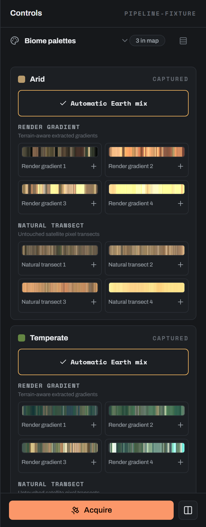
- Climate classes. The authored Köppen crop is matched by colour to its classes and folded into seven macro biomes: tropical, arid, mediterranean, temperate, boreal, tundra and ice. Each macro also carries a mean annual precipitation figure, which is half of what the snow model reads.
- Class blending. Class weights are blurred by Transition width and traded across a dry-to-wet ranking inside the blend bands, so a river crossing a dry boundary pulls green downstream.
- Snow. A mass balance rather than a temperature cut-off: summer temperature against winter accumulation at the equilibrium line, with aspect, avalanching, glacier tongues and sublimation on top. Ground too cold for trees but not under snow paints as bare rock and scree.
- Lakes, when you turn them on. They are off by default. Every depression is then solved for the area its catchment's runoff can hold against open-water evaporation, capped at the spill. Humid basins fill and overflow. Dry ones stop far short of their outlet, and a genuinely closed dry basin renders its floor as a pale evaporite pan. Left off, those depressions are simply dry ground.
- Overlays. Valley darkening, and a beach ring on ocean coasts only. Inland lakes get no ring, because a ring around a lake reads as a halo.
- Native composite. The land and sea cut, the hillshade, the four-zone sea optical model, lake surfaces measured from their solved level and the river channels are all composited at the section's own pixel size.
Two grids, one image#
The look is defined by structure at kilometre scale, so steps 4 to 12 run on the analysis grid. The land mask, the hillshade, the sea optics and the river channels run at native size, which is why coastlines and river threads stay pixel-crisp instead of arriving upsample-smeared. Running the analysis passes at full resolution on a 20,000 px section would cost tens of GB and would not change the look.
Every spatial parameter in the render is denominated in km or km². The two families that would otherwise inherit the working pixel pitch are anchored explicitly: rivers to routed catchment area, and the hillshade to the section's native pitch. Texture detail is therefore a speed and quality trade and nothing else. It no longer moves river width.
When the render degrades#
Nothing degrades silently. Each of these lands as a warning on the finished render:
- No recorded pixel geometry, or no scipy: the section falls back to a plain hypsometric colouring, with no palettes, sea model, snow, rivers or lakes.
- No numba flow kernels: rivers and lakes are off, and the moisture term reverts to the terrain-only proxy.
- No Köppen crop: macro classes are banded from temperature alone. That fallback cannot place arid or mediterranean climates, and it reads any ground at or above 18 °C as tropical, which means 2000 mm/yr of precipitation for the snow and lake models.
The progressive preview#
Every render runs the same pass three times, at 512, 1024 and 2048 px on the long edge, ascending. Each pass publishes a frame the moment it completes, so the canvas sharpens in three steps instead of sitting dark. Progress is weighted by pixel area, so the rungs are 1:4:16 of the bar and the 512 px pass is finished before the bar reaches 5 %.
The steps are capped at the section's native size, so a section under 2048 px reaches native on its last rung.
What the ladder shows you is the final render, approximated. Flow routes from the undownsampled heightmap on every step, so the river network you see at 512 px is the network the final render draws. The hillshade compensates its exaggeration toward the native pitch, so preview contrast moves toward the final image rather than away from it. A channel narrower than one output pixel draws at one pixel with proportional alpha, so more resolution reveals more tributaries without changing the width of the rivers already drawn.
Where the preview stops#
The interactive preview stops at 2048 px. The Output select in the top bar (Native, 2K, 4K, 8K, 16K, 32K) sets the export resolution. It does not change the preview, and changing it does not make the frame stale.
Full-resolution colour comes from two places: an export, or Render section colour, which renders the section at native size and stores the result as the base an AI enhance pass needs.
The adjust loop#
Render, look, adjust, re-render. Dayside has no post-process grade: there is no hue, contrast or temperature control that re-tints a frame after it exists. The colour comes out of the model, so it changes by changing the model's inputs, and that means another render every time.
What marks the preview stale#
Every slider, toggle, colour swatch and palette choice in the render groups marks the current frame stale as soon as you release it. The canvas shows PREVIEW STALE · N CHANGED, where N counts the distinct settings you have moved since the last submitted render, and Acquire becomes Re-render.
In Render mode the panel groups run in this order: Biome palettes, Biome blending, Rivers (with Lakes and Water colour nested under it), Sea, Snow & ice, Global look. Sea and Snow & ice each carry a Reset button in the group header that returns that group to the world's defaults, marking stale only the values that actually moved.
Palette preferences behave slightly differently: they are saved to the world's manifest as you reorder them, and the save is what marks the frame stale.
What costs nothing#
- Compare, in the top bar and in the panel footer. It wipes the previous frame against the current one, tagged A · PREVIOUS and B · CURRENT. Drag the divider.
- Panning, zooming (0.6× to 3.0×) and Fit.
- The Output select.
- The guide overlay and its opacity.
- Switching to Draw mode and back.
What costs more than a re-render#
- Generate re-synthesises the heightmap on the GPU, then triggers a colour render of its own.
- Enhance section colour runs a learned pass on the GPU and needs a persisted native analytic render first.
- Export re-renders every requested layer at the export resolution. A satellite layer is roughly eight times the cost of re-encoding a mask.
Getting a result you like#
Most of the image is decided by a handful of controls. Reach for these first. Every remaining parameter, with its full range and its interactions, is in Colour and climate reference.
| Control | Engine key | Default | Range | What it does |
|---|---|---|---|---|
| Relief | hillshade_exag | 3.0× | 0.5 to 6× | Vertical exaggeration of the hillshade. Changes how steep the terrain reads. |
| Relief shading | hillshade_strength | 100 % | 0 to 100 % | Opacity of that shading. 0 % skips the hillshade pass entirely. |
| Transition width | koppen_blur_km | 25 km | 0 to 80 km | How far two climates blend into each other. |
| Density | river_min_catchment_km2 | 25 km² | 1 to 400 km² | Smallest catchment that draws as a river. Slider is inverted: right is denser. |
| Width | river_width_km | 150 m | 20 to 600 m | Drawn width at a 10,000 km² catchment. Every channel scales as √catchment from there. |
| Snow line | t_snow_c | -2.0 °C | -12 to +8 °C | Bias on the model's critical temperature. Higher is warmer, so more snow, lower down. |
| Warmth | t_lat0_c + t_eq_c | 0 °C offset | ±15 °C | Shifts the whole temperature field. Moves vegetation, snow and lake evaporation together. |
| Dryness | lake_evap_scale | ×1.00 | 0.25 to 4× | Scales net evaporation on closed basins. Above 1 is drier: smaller lakes, more playa. |
| Texture detail | analysis_long_side | 4096 px | 1024 to 8192 px | Analysis grid long side. Cost and quality only. |
Relief and relief shading#
These two are separate and they are not interchangeable. Relief changes the pattern of the shading; Relief shading changes how much it darkens.
The trap is treating Relief as an on and off switch. Low exaggeration does not remove shading, it flattens the gradient toward a near-uniform multiply that brightens the whole frame and clips pale ground. At zero exaggeration, which the API allows even though the slider floors at 0.5, every land pixel is multiplied by about 1.08 and anything already above 0.926 (snow, ice, sand, pale sediment) blows out to flat white. That is an over-exposed image.
To take the shading off, put Relief shading at 0 %. That skips the hillshade pass completely, which is also a real memory and time saving on large sections: the pass holds around 6.2 GB of transient at 16K.
Rivers#
Density sets the smallest rain-weighted catchment that draws as a river, in km². The slider is inverted, so dragging right lowers the threshold and gives a busier network. The 25 km² default is a well-drained landscape; push toward 400 km² for trunk rivers only.
Width is the drawn width at a 10,000 km² catchment, and every channel scales as the square root of its own catchment from that anchor. 150 m is satellite-honest, Thames-class. 300 to 500 m is cartographic emphasis, legible when you pull back to a globe view. Width is capped at 12 km as a runaway guard for continental basins, so treat that as a ceiling you should never approach.
If your rivers read as pale threads at distance, raise Green banks (riparian_green, default 0.15) before you raise Width. The green vegetation ribbon along a watercourse is what makes it legible when the thread itself is pale, and river colour is keyed to climate: dry climates get a river lighter than the land around it, wet and cold climates get a darker one.
Turning Rivers off takes lakes with it and greys out Flow widening, Green banks, River strength and every lake control. Those parameters are inert without routing, because there is nothing routed for them to read.
Climate transitions#
Transition width is the strongest single control over how the image reads from a distance. The 25 km default gives a boundary that is soft but still defined. Wide values with the dither off airbrush a border into a wash.
It is silently capped at about 10 % of the section's extent. When your value exceeds the cap the slider shows an amber CAPPED AT n KM ON THIS MAP note, and anything above it does nothing. A focus area cut from a coarse world raster can also come out wider than you asked, because the blur is widened to at least 1.5 cells of the source climate raster to melt its nearest-neighbour staircase.
Patchiness (ecotone_dither) defaults to 0 and tops out at 0.15. That ceiling is deliberate: higher values broke the crossfade into a green and tan camouflage mosaic. Use 0.05 or less for a whisper of grain.
Snow line and warmth#
Snow is solved as a mass balance, so it responds to precipitation as much as to temperature. A wet maritime range carries perennial snow far lower than a dry continental plateau at the same temperature, which is the behaviour you want and also the reason the controls do not feel like a simple elevation cut.
Snow line biases the model's critical temperature. Higher is warmer, which means more snow reaching lower ground. The panel prints an approximate figure in km underneath at 6.5 °C/km, along with a reminder that authored Köppen climate takes precedence over the latitude estimate. Coverage (t_width_c, default 3.0 °C) softens the edge of the transition. Snow shedding (snow_slope_deg, default 50°, under Advanced) is the centre of the avalanche band: nothing perennial survives above about 55°, all of it survives below about 35°.
Warmth moves t_lat0_c and t_eq_c together by up to ±15 °C, which shifts vegetation, snowline and lake evaporation at once. It is the biggest lever in the group, so move it in small steps.
One measurement trap worth knowing: frame brightness is not a proxy for snow coverage. Ground too cold for trees but not under snow renders as bare rock, so widening the snow band can make the frame darker.
The sea#
Deep cutoff (default 45 m) is the depth at which the seabed stops being legible and the water goes to a uniform deep colour. Raise it and shelves read further offshore; keep it low and the coast reads like a photograph. Below the cutoff there is no bathymetry legibility at all, on purpose: a kilometres-deep colour ramp reads as a drained basin.
With Tint shallows by biome on, shallow water is keyed to the climate of the adjacent coast, and Coast blend (sea_biome_blur_km, default 25 km) sets how far two climates mix across a shared bay. Coast blend does not move river colour; river tint is always blurred at 25 km regardless of what you set here.
Texture detail and seed#
Texture detail labels itself Draft at or below 2048, Balanced at or below 4096, Fine at or below 6144 and Maximum above that. Drop to Draft while you are dialling in climate, snow and lakes, then put it back to Balanced or higher for the version you keep.
Seed (default 7) re-rolls the procedural fields: the mid-frequency mottling, the lithology provinces and the ecotone dither. Terrain and climate are untouched. Each field draws from its own child generator, so re-seeding one subsystem never re-phases another field's geography.
One cap to know about: a small section genuinely cannot show a macro biome's full material spread. The number of surviving material variants per macro is set by the section's extent against the province scale, so a 200 km section at the default 160 km province scale gets one variant per macro no matter how many the palette bank holds.
Enhance section colour#
Enhance section colour adds learned high-frequency satellite detail to the analytic render. It works on luminance; hue and water stay analytic. It runs on the packaged NVIDIA model, on the GPU, in its own modal from the top bar.
It is an optional add-on that ships separately from the app. If your installation does not have it, the modal says so and repairing or reinstalling will not add it.
What it needs first#
The pass needs a persisted, native-resolution analytic colour render, because it slices that colour PNG and the signed heightmap on the same native grid. The interactive preview ladder does not produce one: it stops at 2048 px and publishes preview frames.
When it is missing, the modal offers Render section colour. That runs a separate, cancellable job that renders the section at native size and commits the result. It can take a few minutes. Colour globe does not satisfy this either; it builds the world mosaic and never renders a section's analytic colour.
Running the pass#
Detail strength runs from 0.05 to 1.00 in steps of 0.05, default 0.40. The result replaces the frame on the canvas, and Compare switches its tags to A · ANALYTIC and B · LEARNED DETAIL so you can wipe the two against each other.
Only one enhance result exists per section at a time. Use Reset to analytic before running another pass at a different strength.
On first run the modal may ask to download the SD1.5 base model. Dayside ships only its own trained adapter. The base model is fetched once from its publisher at a pinned revision, every byte is verified against hashes built into the app, and the CreativeML OpenRAIL-M licence has to be accepted before the download starts.
Keeping the result fresh#
An enhance result is fresh only while the analytic base it consumed is still on disk and still hashes to the same bytes. Any new colour render invalidates it, and the canvas drops the comparison.
That freshness rule reaches the export modal. Satellite colour · enhanced ships only a fresh result and refuses the layer rather than substituting the analytic image. The separate Compose Enhance section colour into the satellite layer toggle is more forgiving: it falls back to the analytic colour with a warning if nothing fresh exists.
After the render#
A finished frame is a preview. To get files, use Export for this section, or fold the section back into the planet and export the globe. Exports queue like renders, land in the Acquisitions drawer with a receipt listing every file and its size, and a section export caps at 16384 px while a world export caps at 32768 px.