Colour and climate reference
Every parameter the colour render reads: defaults, ranges, engine keys, the silent caps, and which controls go inert.
This is the complete parameter surface of the satellite colour render. It covers what each control writes, what the engine does with it, where a value is silently clamped and where a slider does nothing at all. For how to actually drive a render, read Rendering the satellite image. For the physics behind the numbers, the summaries here are enough to tune by.
Reading the tables#
Every table uses the same columns.
- Control is the on-screen label in the Controls panel, exactly as it appears. Rows marked
not exposedhave no control and are reachable only over the API. - Engine key is what travels on the wire. Unless a row says otherwise the key goes inside
paramsonPOST /api/worlds/{id}/renders. A few are top-level render fields (style,hillshade_exag,analysis_long_side,rivers,seed) and the sea model is its ownseaobject, written assea.<field>. - Default is the shipped value.
GET /api/worlds/{id}/defaultsreturns the live set that the panel loads, pluskoppen_blur_cap_kmfor this section. - Range is the UI slider range where a slider exists, and the wire bounds where they differ. The API bounds-checks a fixed list of keys and returns 422 outside it. Keys outside that list accept any finite JSON number and are marked
not bounds-checked.
Three things apply to the whole page.
Only the satellite style reads any of this. The hypsometric, atlas and spectral styles ignore palettes, the sea model, snow, rivers and lakes, and the engine warns if you ask for the unlit or water outputs on them.
The API accepts any scalar key of the engine's DEFAULT_PARAMS, including keys with no slider. Four tuple-valued keys (wet_radii_km, wet_weights, cav_radii_km, cav_weights) are engine-only and cannot be sent over the wire at all.
Every spatial parameter is in km or km², converted at the working pixel pitch. Anything finer than one pixel of that grid cannot be drawn. See Silent caps in one place.
Sea level and water#
Sea level is a datum#
Sea level is 0 m by definition in the signed heightmap: land positive, ocean negative. The render does not have a sea-level slider because there is nothing to set. What exists is a datum control in Draw mode, under Height brush, which rebases the whole field and rewrites the heightmap.
Moving it live-updates the preview and commits on release. At either endpoint the panel warns that you are about to produce an all-land or all-sea map with no usable coastline. After a model Generate it warns that changing sea level reclassifies model-authored land and ocean, and advises setting it before Generate instead.
| Control | Engine key | Default | Range | What it does |
|---|---|---|---|---|
| Sea level (Draw mode) | sea_level_norm on POST /api/worlds/{id}/terrain/commit | 0.50 | 0 to 1, step 0.01 | Rebases the section's height datum. The response reports the applied sea_level_offset_m. |
not exposed | sea_level_m (engine kwarg) | 0.0 m | not bounds-checked | Rebases the elevation field inside the colour engine. The server render path always leaves it at 0, because the signed heightmap is already sea-relative. Not reachable through the render API. |
The four-zone sea optical model#
Water is rendered as a satellite sees it. Four depth anchors carry a colour and a seabed-legibility figure: transparent turquoise over visible bed at 0 m, the bed fading through saturated cyan into medium blue by 25 m, a ghost of it at 45 m, and below that a uniform inky deep with zero bathymetric legibility. That last zone is deliberate. A colour ramp that keeps describing depth for kilometres reads as a drained basin.
Deep cutoff is the lever for shelves that read too brightly. Pulling it below 45 m compresses the shallow anchors along with it, so the turquoise reaches a shorter way down and covers less of the map. The three seabed visibility figures under Advanced are the other half of the same job: they set how much lit bed shows through the water at each anchor, and lowering them mutes the texture without moving the colour.
Omitting the sea object entirely is pixel-identical to the defaults. The Reset button in the group header restores every sea field and also puts Coast blend back to its default.
| Control | Engine key | Default | Range | What it does |
|---|---|---|---|---|
| Tint shallows by biome | sea.tint_shallows_by_biome | on | on or off | Keys shallow water to the climate of the adjacent coast. Off gives one global shallow, mid and bed tint. |
| Deep cutoff | sea.depth_anchors_m[3] | 45 m | 10 to 200 m | Depth at which the seabed stops being legible and the water goes uniform, in clear water. Every coast divides it by its own sea.clarity_by_macro, so 45 m is what a tropical shelf gets and a boreal one loses its bed by about 13. Below 45 m the two shallow anchors compress with it, so the whole shallow ramp lands in a shorter depth range. |
| Deep water colour | sea.water_colors[3] | #112339 | any #RRGGBB | The open-ocean colour below the cutoff. Anchored on measured Sentinel-2 cloudless ocean, then darkened. |
| Shallow tint | sea.water_colors[0] | #8fd0cf | any #RRGGBB | The global 0 m colour. Only shown when biome tinting is off. |
| Coast blend | sea_biome_blur_km | 25 km | 0 to 100 km | Blur on the biome-keyed shallow-water fields, so bays blend where two climates share a coast. Inert, and greyed out, when biome tinting is off. |
| Shallow seabed visibility | sea.bed_visibility[0] | 0.70 | 0 to 1, floored at the mid value | Seabed legibility at the 0 m anchor. |
| Mid seabed visibility | sea.bed_visibility[1] | 0.38 | clamped between its two neighbours | Legibility at the 5 m anchor. |
| Lower seabed visibility | sea.bed_visibility[2] | 0.06 | 0 to the mid value | Legibility at the 25 m anchor. |
| Tropical shallow tint and six more | sea.shallow_by_macro | 7 hexes | #RRGGBB each, all 7 macros required | Per-climate 0 m colour. Tropical is a clear carbonate bank, temperate a murky grey-green shelf, ice a milky glacial one. |
not exposed | sea.depth_anchors_m[0..2] | 0, 5, 25 m | four increasing anchors starting at 0 | The shallow anchors. Held at their defaults for any cutoff of 45 m or more, and scaled by the cutoff below that. The panel prints the live values under Advanced as a read-only note. |
not exposed | sea.mid_by_macro | 7 hexes | all 7 macros required | Per-climate colour at the 5 m anchor. |
not exposed | sea.beach_by_macro | 7 hexes | #RRGGBB each, all 7 macros required | Beach and seabed base colour, keyed to the adjacent coast's climate. White carbonate sand is a tropical phenomenon: temperate is grey-brown shingle, boreal dark cobble, ice pale rock flour. Feeds both the land beach ring and the lit bed seen through the shallows, so the sea toggle below does not govern it. |
not exposed | sea.clarity_by_macro | 1.0 tropical and arid, 1.3 medit, 2.5 temperate, 3.5 boreal, 3.0 tundra, 2.5 ice | above 0 to 20, all 7 macros required | Multiplies the depth the optical model sees, so the cutoff is per climate: effective cutoff = sea.depth_anchors_m[3] divided by clarity. Plankton and river silt scatter the light out of a temperate shelf by about 18 m and a boreal one by about 13. Above 1 is murkier, below 1 clearer. |
not exposed | sea.bed_tint_by_macro | 7 RGB triples | 0 to 1 per channel, all 7 macros | Multiplies that climate's beach colour to give each one its own seabed. |
not exposed | sea.bed_visibility[3] | 0.0 | must be exactly 0 | The deep zone. Fixed, and the panel labels it DEEP VISIBILITY: 0 (FIXED). |
Only the 0 m and 5 m anchors, the beach and seabed colour, and the clarity multiplier vary per climate. The anchor depths themselves and the deep colour stay global: clarity changes the depth those global anchors are read at, not the anchors. Everything depth-dependent is folded into 256-entry lookup tables indexed at native resolution, so a shelf edge stays pixel-crisp. Class assignment extends over water by filling from the nearest land class, so shallow water needs no separate coast lookup. A frame with no land at all falls back to the tropical set.
The deep sea is the only part of the image the hillshade does not touch. The shallow seabed ghost is lit.
The beach ring#
| Control | Engine key | Default | Range | What it does |
|---|---|---|---|---|
not exposed | beach_km | 1.0 km | not bounds-checked | Width of the beach ring. Ocean coasts only. |
not exposed | beach_zmax_m | 40.0 m | not bounds-checked | Elevation past which the beach stops. |
Inland lakes get no beach ring, on purpose. A ring around a lake reads as a halo rather than a shore. The ring is also under-resolved below about one pixel of the analysis grid: on a 1000 km section at a 512 px grid the default 1.0 km is 0.51 px wide and simply fades out. That is expected behaviour.
The water mask#
water_mask is a shipped export layer, filled from the same composite traversal as the colour, so it costs almost nothing. Values are 255 for standing water (ocean plus solved lakes), the anti-aliased coverage times 255 for river channels, and 0 for dry land. Playa pans read as dry. Standing water wins wherever the two overlap.
Do not conflate it with sea_mask. sea_mask states the heightmap decode contract, which is z <= 0. water_mask states where water actually stands. It is the shipped superset of the still-deferred river_mask, and it is section-only, because the globe pass routes no flow.
Climate: temperature, lapse rate and rainfall#
Temperature is built from a latitude curve, a continentality shift derived from distance to the ocean, and a free-air lapse rate. The curve needs both the section's centre latitude and its extent. Without them the section is unlocated: it takes a uniform t_eq_c, and it has no seasonal swing at all, so summer equals the annual mean. That is the honest reading of not knowing where the ground is.
The Warmth slider under Snow & ice is the only exposed temperature control, and it moves two keys together. Reset on that group restores both, along with the three snow keys.
| Control | Engine key | Default | Range | What it does |
|---|---|---|---|---|
| Warmth | writes t_lat0_c and t_eq_c as default + offset | 0 °C offset | -15 to +15 °C, step 0.5 | Shifts the whole temperature field. Moves vegetation, the snow line and lake evaporation together. |
| Warmth (component) | t_lat0_c | 27.0 °C | wire 12 to 42 °C | Equatorial sea-level mean annual temperature of the latitude curve. |
| Warmth (component) | t_eq_c | 22.0 °C | wire 7 to 37 °C | Uniform fallback temperature used when the section has no projection metadata. |
not exposed | t_lat_drop_c | 23.0 °C | not bounds-checked | The sin² term of the latitude curve. |
not exposed | t_lat_drop4_c | 22.0 °C | not bounds-checked | The sin⁴ term. Together with the pair above this reproduces 27, 20, 10, -1, -12 and -18 °C at 0, 30, 45, 60, 75 and 90 degrees. |
not exposed | lapse_c_per_km | 6.5 °C/km | not bounds-checked | Free-air lapse rate. Read by both the colour pass and the snow model. |
Continentality shifts the mean about that zonal average and is centred on 0.5, so interiors fall below the zonal figure as far as maritime coasts rise above it. At the pole the full continental chill is 14 °C, scaled by sin² of latitude. It also widens the seasonal swing, which is what the snow model reads.
Rainfall#
The colour render has no rainfall parameter. Rainfall reaches it two ways.
A rainfall layer attached to the world weights the flow accumulation. Weights are normalised to a land mean of 1, so a desert basin accumulates less than its geometry alone would give it. Missing rainfall means uniform runoff, which is a graceful degradation and not an error. The physical scale comes from the mm/yr at white you recorded when you attached the map, which is why that number matters: get it wrong and nothing breaks visibly.
Everything else comes from the climate classes. Each macro carries one mean annual precipitation figure, listed in The seven macros, and that figure is half of the snow model.
Rivers and flow routing#
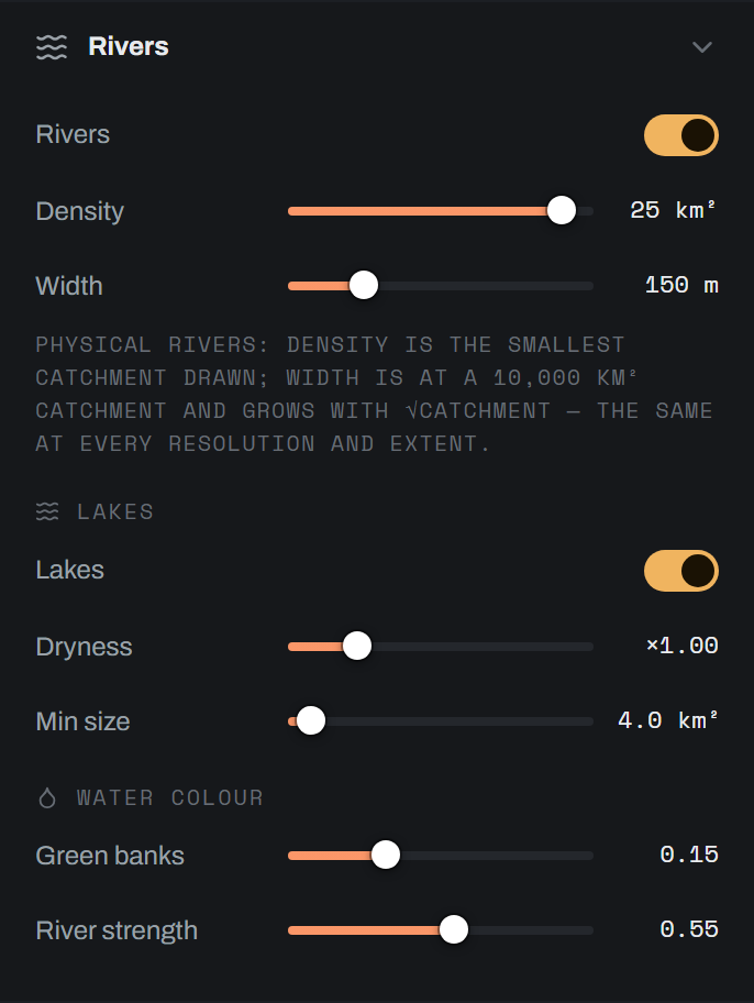
Rivers are physical. Which cells are rivers is an absolute threshold on rain-weighted upstream catchment in km². How wide each channel draws is hydraulic geometry: w = river_width_km × √(A / 10,000 km²). Both are denominated in physical units, so the network is identical at every preview step, every analysis resolution and every section extent. The visible signature of changing resolution is more tributaries appearing, never rivers getting fatter or thinner.
| Control | Engine key | Default | Range | What it does |
|---|---|---|---|---|
| Rivers | rivers (top-level render field) | on | on or off | Runs the flow routing and passes its fields to the renderer. Off takes lakes with it and makes six other controls inert. |
| Density | river_min_catchment_km2 | 25 km² | UI 1 to 400 km², wire 1 to 5000 | The smallest rain-weighted catchment that draws as a river. The slider is inverted: right is a lower threshold and a busier network. |
| Width | river_width_km | 0.15 km, shown as 150 m | UI 0.02 to 0.6 km, wire 0 to 2 | Drawn width at a 10,000 km² catchment. 150 m is satellite-honest, Thames-class. 300 to 500 m is cartographic emphasis. |
| River strength | river_blend | 0.55 | 0 to 1 | How strongly a channel blends the land colour toward the climate river tint. At 0 no channel is drawn and the water mask reports standing water only. |
| Green banks | riparian_green | 0.15 | 0 to 0.5 | The green vegetation ribbon along a watercourse. The channel gain is weighted (0.4, 1.0, 0.25) across red, green and blue, so it greens far more than it brightens. 0 disables it. |
Flow-routed wetness#
The routed drainage replaces most of the terrain-only moisture proxy wherever the terrain genuinely drains, and hands back to the proxy inside depression fills, where routed values mislead in both directions.
| Control | Engine key | Default | Range | What it does |
|---|---|---|---|---|
not exposed | flow_blend | 0.7 | not bounds-checked | How much routed drainage replaces the proxy in the wetness term. Multiplied by the depression-fill trust field. |
not exposed | flow_wet_blur_km | 2.0 km | not bounds-checked | Riparian blur on the wetness copy of the flow. Vegetation responds over km while the channel itself stays sharp. |
not exposed | lake_fill_m | 2.0 m | not bounds-checked | Depression-fill depth past which routed values are distrusted. Trust ramps down between this and three times this. |
not exposed | base_flow | 0.10 | not bounds-checked | Raw routed flow as a streaky drainage tint in the texture base, unblurred on purpose. Inert without rivers. |
River colour is keyed to climate#
River tint is a module constant with no parameter behind it. Dry climates get a river lighter than the land around it and wet or cold climates get a darker one, which is why the same River strength slider does both.
| Macro | Tint | Reads as |
|---|---|---|
| tropical | #8a744c | Amazon café-au-lait |
| arid | #dccba1 | Sahel pale warm sand, lighter than the land |
| medit | #cdbc93 | pale sediment |
| temperate | #55604c | green-grey water |
| boreal | #3f463a | tannin-dark |
| tundra | #a7a8a4 | glacial rock flour |
| ice | #bcc7cc | meltwater steel |
The tint field is blurred at the default 25 km regardless of what you set Coast blend to. That control deliberately does not move river colour.
Caps and gates on rivers#
Width is capped at 12 km. That is a runaway guard for continental basins and not a tuning knob, so treat it as a ceiling you should never reach.
A channel narrower than one output pixel draws at 1 px with alpha equal to its width over the pixel pitch, rather than saturating to a full pixel. That sub-pixel floor is what keeps the same network honest from a 5 km/px preview to a 20,000 px native render.
Cells whose depression-fill depth is at or above three times lake_fill_m, so 6 m by default, never seed channel geometry, and the wetness term reverts to the proxy there.
river_width_km = 0 renders. The wire range floors at 0 while the slider floors at 0.02 km, and it is not clear from the code whether that draws no channel at all, or a sub-pixel channel that still carries Green banks.Drainage entering from a neighbouring section is approximated by splicing a ring of the authored world canvas around the section before routing. If the ring's brightness-to-metres calibration fails to fit, no splice happens at all. Either way, trunk catchments inside a section are floors: a continental river entering the frame draws at the width its truncated catchment supports.
Lakes and the endorheic balance#
A lake is solved as a mass balance. A depression does not simply fill to its rim. Per basin:
A_eq [km²] = Q [km²] × R [mm] / E_net [mm]
E_net = (PET_lake - P) × lake_evap_scale, floored at 50 mm
Q is the peak routed catchment inside the basin. R is Budyko-Fu runoff, which is the term that kills the arid-basin lake: a desert catchment yields a few mm of runoff from hundreds of mm of rain, and no amount of rain-weighting the accumulation can express that. PET_lake is open-water potential evaporation, 450 × exp(T / 15) mm/yr. Where PET <= P the basin is humid: it fills to its spill and overflows, and the routed rivers already continue downstream.
The solver then walks the basin's hypsometry and takes the level whose flooded area reaches A_eq, capped at the spill. Against Earth this puts the Caspian at a lake-to-catchment ratio of 0.106 against a real 0.103, the Great Salt Lake at 0.071 against about 0.08, the Dead Sea at 0.021 against about 0.024, and Lake Eyre at 0.002, which is to say dry.
| Control | Engine key | Default | Range | What it does |
|---|---|---|---|---|
| Lakes | lakes | 0.0 (off) | 0 to 1 | Master gate on the standing-water solve. Off, a closed depression is dry ground rather than a lake; it does not flood anything back as sea. Greyed out when Rivers is off. |
| Dryness | lake_evap_scale | ×1.00 | 0.25 to 4 | Scales net evaporation. Above 1 is drier, giving smaller and fewer lakes and more playa. Below 1 is wetter. The one taste dial in the group. |
| Min size | lake_min_area_km2 | 4.0 km² | 0.5 to 100 km² | Absolute area floor. Resolution-invariant by construction, and the reason you do not get thousands of pixel ponds. |
not exposed | lake_min_depth_m | 2.0 m | not bounds-checked, and not in the defaults response | A solved lake shallower than this at its deepest is not drawn. |
not exposed | playa_blend | 0.85 | wire 0 to 1 | Opacity of the evaporite-pan tint on dry closed-basin floors. It is in the defaults response and bounds-checked, but there is no slider for it. |
Enclosed pockets route as land#
Whenever the flow routing runs, ocean means cells below 0 m that connect to the border of the routing grid, plus any cell the authored world canvas declares ocean that is still below 0 m after generation. Everything else below 0 m is an enclosed pocket, and a pocket routes as land. The priority flood then measures the whole depression and the accumulation threads its inflow to the spill.
This is not tied to the Lakes toggle. Pockets route as land either way; Lakes decides only whether the mass balance then puts water in them. With Lakes off you get dry basins, not inland seas.
The author's statement outranks the physics. An authored inland sea stays a sea. A pocket a diffusion model happened to invent is not a statement, so it is treated as ground until the balance says otherwise. Generated land that rose above 0 m has moved the shore and stays land. A pocket touching the grid border cannot be told from a truncated sea and conservatively reads as ocean.
In the renderer those pocket cells are land to every analysis stage, including climate, colour and snow, and their floors take sea-level temperatures. That is the Death Valley reading, and it is intended.
Playa pans#
A basin that is genuinely closed (it did not spill), has at least 4 m of relief between floor and spill, and is arid enough to crust, renders its floor as a pale evaporite pan when its solved lake is absent or pruned. A shrunken terminal lake keeps a pan ring around it. The pan colour is #e8e1cd, brighter than any arid land ramp so a dry lake reads as its own feature, but deliberately not pure white, which would read as snow.
The pan is painted before the snow blend, so a cold playa snows over like any other ground. In the water mask a playa is dry.
Engine constants for the balance#
These are module tuning. None of them can be set from anywhere.
| Constant | Value | What it is |
|---|---|---|
PET_REF_MM | 450.0 | Open-water potential evaporation at 0 °C. |
PET_EFOLD_C | 15.0 | Its e-folding temperature. |
FU_OMEGA | 2.6 | Budyko-Fu shape. Higher means more evaporation and less runoff. |
E_NET_MIN_MM | 50.0 | Net-evaporation floor. Basins at this floor are near-humid, so the spill cap does the real work. |
REGIONAL_KM | 60.0 | Blur on the climate fields read at a basin. Runoff is generated over the catchment, and a terminal lake is usually the driest spot in its own basin. |
BASIN_MEMBER_M | 0.01 | Fill depths at or under this are epsilon-fill noise. |
BASIN_MIN_RELIEF_M | 0.5 | A basin shallower than this end to end can never pass the depth floor. |
PLAYA_RELIEF_MIN_M | 4.0 | Minimum spill-to-floor relief for a playa. |
PLAYA_FLOOR_BAND_M | 2.0 | The pan wets the floor plus this band. |
PLAYA_ARIDITY_PHI | 1.5 to 4.0 | The aridity smoothstep band grading pan strength. |
Frozen lake surfaces are future work. A lake in a cold climate currently renders with the same water optics as any other.
Snow and ice#
Perennial snow exists where a year's accumulation survives a year's ablation, so the governing quantities are summer temperature, which melts, and winter accumulation, which does not. The two trade off against each other. That is why Patagonian and Norwegian glaciers reach sea level at 46 to 60 degrees while the Tibetan Plateau at 5000 m is largely bare, and why the Dry Valleys sit ice-free inside Antarctica.
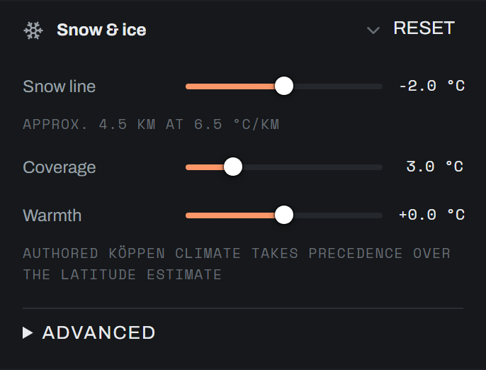
The chain runs continentality, summer temperature, accumulation, the Ohmura equilibrium-line condition P = 645 + 296T + 9T², aspect as an integrated direct-radiation ratio, avalanching, glacier tongues, and finally the nival zone.
| Control | Engine key | Default | Range | What it does |
|---|---|---|---|---|
| Snow line | t_snow_c | -2.0 °C | -12 to +8 °C, step 0.5 | Bias on the model's critical temperature. Higher is warmer, so more snow reaching lower ground. |
| Coverage | t_width_c | 3.0 °C | 0.5 to 12 °C, step 0.5 | Softness of the smoothstep on the gap between critical and effective summer temperature. |
| Snow shedding (under Advanced) | snow_slope_deg | 50° | 20 to 80° | Centre of the avalanche band. Nothing perennial survives above centre plus 5°, all of it survives below centre minus 15°, which is the textbook 35 to 55 degree window at the default. |
| Warmth | t_lat0_c and t_eq_c | 0 °C offset | -15 to +15 °C | Shared with the climate group. Shifts the whole temperature field. |
not exposed | lapse_c_per_km | 6.5 °C/km | not bounds-checked | Read by the model to cool peaks. |
Snow line is a bias now#
Snow used to be a single smoothstep on mean annual temperature and t_snow_c used to be that threshold. It is now a bias applied to the Ohmura critical temperature, with the neutral point at -2.0 °C, which is why the default is exactly the neutral value. The slider direction is unchanged: higher is a warmer line and more snow. The panel prints an approximate km figure underneath at 6.5 °C/km, derived from the gap between t_lat0_c and t_snow_c. Treat it as an indicator rather than an elevation you can rely on, because the model does not use a single elevation anywhere.
Snow shedding is judged on resolution-compensated slope in tan-space, so the angle means the same thing at 30 m/px and at 700 m/px.
Reading a snow render#
Two things surprise people.
Frame brightness is not a proxy for snow coverage. Ground too cold for trees but not under snow is bare rock and scree, drawn from its own rock ramp (#544c45 to #b3a898), so widening the snow band can render darker. Snow and rock partition by construction: they sum to at most 1, so it is one blend rather than two stacked overlays.
Climate reaches the model through two different blurs, and this is deliberate. Temperature and the authored-ice cap take a tight blur, just enough to melt the Köppen source's staircase. Precipitation takes the wide ecotone blur, because moisture is regional: it arrives on the wind and is wrung out over whatever terrain it meets. Sharing either blur breaks the model. Measured on a 3 km-pitch crop, an EF massif's class weight fell to 0.21 under the wide blur, which turned its -4 °C cap into +3.3 °C and melted the ice sheet clean off it.
The model is pinned against 13 real ranges with published snowlines: Spearman rho about 0.97, mean bias about -50 m, mean absolute error about 590 m.
Biomes and Köppen classification#
Classification has one parameter. Everything else is authored, either by uploading a Köppen-coloured climate map at setup or by painting classes with the biome brush.
| Control | Engine key | Default | Range | What it does |
|---|---|---|---|---|
not exposed | koppen_src_pitch_km | 0.0 | not bounds-checked | The true information pitch of the authored Köppen source, in km per source pixel. The render derives it from the crop rectangle against the extent and injects it; a value you send overrides that. Above 0 it widens the class blur to at least 1.5 source cells, which melts the nearest-neighbour staircase a focus-area crop inherits. |
The authored crop is matched to Köppen classes by colour, over the raster's unique colours rather than every pixel, with a single RGB euclidean tolerance of 60. One tolerance is shared by the palette-file present-class filter and the per-pixel matcher on purpose: two different thresholds would strand classes in between, admitted as present but never matched, so their territory backfills from neighbours.
Pixels further than the tolerance from any palette colour, and pixels where all channels exceed 240 (a white background), classify as unknown and then fill from the nearest known class. A palette with duplicate colours resolves to the first matching code in the canonical order; the loser is a legitimate zero-pixel class. The class masks you export cut on exactly the same boundaries the colour render used, because both go through the same matcher.
The seven macros#
Every Köppen class folds into one of seven macro classes. Each macro carries a gradient bank, a sea-level mean annual temperature floor and one precipitation figure.
| Macro | Köppen classes | Sea-level floor | Precipitation |
|---|---|---|---|
| tropical | Af, Am, Aw, As | 20 °C | 2000 mm/yr |
| arid | BWh, BWk, BSh, BSk | 12 °C | 150 mm/yr |
| medit | Csa, Csb, Csc | 10 °C | 550 mm/yr |
| temperate | Cwa, Cwb, Cwc, Cfa, Cfb, Cfc | 6 °C | 1000 mm/yr |
| boreal | Dsa to Dsd, Dwa to Dwd, Dfa to Dfd | 0 °C | 550 mm/yr |
| tundra | ET | -6 °C | 250 mm/yr |
| ice | EF | caps at -4 °C, and at -5 °C in the ablation season | 200 mm/yr |
Those floors are why an authored world does not obey Earth's latitude. On an authored world the climate layer outranks the latitude curve: a temperate zone at 60 degrees south must not render snowbound because Earth's curve says so. The lapse rate still cools peaks into alpine snow. Ice is the mirror image and caps rather than floors, and it caps summer as well as the mean, because a mean-annual cap alone would let an EF zone at 45 degrees melt straight out through its roughly +9 °C seasonal swing. Aspect, lapse and avalanching still cut nunataks and bare faces into an ice cap, which is the difference between a climate and a paint bucket.
The floors are gathered through the softened class weights rather than a nearest-neighbour argmax, so a snow line crossing a climate border follows the terrain instead of the source raster's cells.
Tundra and ice get one more correction. Both say almost nothing about moisture supply, since they occur in polar deserts and on soaking maritime mountains alike. Their 250 and 200 mm figures are the polar reading, and applying them to an alpine cap starves the glaciers the class was authored to imply. So the precipitation blend is taken over the regional, non-alpine classes present in the frame, and only falls back to the polar values when there is no regional climate at all, which is a genuine ice sheet.
The no-Köppen fallback#
With no authored climate the render classifies from temperature alone, which is latitude and altitude banding and nothing else:
| Temperature | Macro |
|---|---|
| 18 °C and above | tropical |
| below 18 °C | temperate |
| below 7 °C | boreal |
| below -2 °C | tundra |
| below -8 °C | ice |
It cannot place arid or mediterranean climates at all, because those need a moisture model. State the consequence to yourself before you tune anything: a world with no Köppen layer reads every patch of ground at or above 18 °C as tropical, which means 2000 mm/yr of precipitation. That is very wet for both the snow model and the lake balance, and it will make lakes fill and glaciers reach low. Authoring a Köppen layer is the intended path.
Biome blending and ecotones#
Transition width is the strongest single control over how the image reads at a distance. There is deliberately no domain warp anywhere in the pipeline; shapes come from the authored classification and the physical fields only.
| Control | Engine key | Default | Range | What it does |
|---|---|---|---|---|
| Transition width | koppen_blur_km | 25 km | 0 to 80 km | Blur on the class weights. Silently capped at about 10 % of the section extent. |
| Flow widening | ecotone_widen | 3.5 | 1 to 8, step 0.1 | The wider blur multiple that riparian flow lerps toward, so transitions widen where water flows. Inert, and greyed out, when Rivers is off. |
| Wet bias | ecotone_k | 0.6 | 0 to 1.5 | Strength of the dry-to-wet weight transfer inside blend bands. A river crossing a dry boundary pulls green downstream, which is the Nile effect. |
| Patchiness | ecotone_dither | 0.0 | 0 to 0.15 | A km-scale noise threshold that breaks the crossfade into a mostly-single-class mosaic. Default off. |
| Patch size | ecotone_dither_km | 13 km | 2 to 40 km | Patch size of that mosaic, softened by a fixed 1 px blur. |
The Patchiness ceiling of 0.15 is a hard invariant in both the UI and the API. A value of 0.65 once scattered tan and green palettes across a wide blur and produced a camouflage mosaic. Use 0.05 or less if you want a whisper of grain, and leave it at 0 otherwise.
The transfer ranks climates from driest to wettest as arid, medit, tundra, boreal, temperate, tropical. Ice sits out of the ranking entirely, because snow is painted by the mass-balance model rather than traded between classes.
Two things can move Transition width away from the number on the slider. The extent cap clamps it downward, and the panel then shows an amber CAPPED AT n KM ON THIS MAP note. The source-pitch widening pushes it upward, silently, on a focus crop taken from a coarse world raster. Both are described in Silent caps in one place.
The texture base#
One greyscale field indexes every climate gradient. 0 is the dry, bare end of a climate's material ramp and 1 is the wet, lush end.
B = clip(0.5
         + base_wet  × (wetness - 0.5)
         - base_slope × slope
         + base_cav  × concavity
         + geo_amp   × geology
         + base_chaos × chaos
         - base_ridge × ridge
         + jitter    × noise
         + base_flow × flow
         - base_cav_fine × fine_convexity
         + base_drain × drainage_proximity,
         0, 1)
Three of these terms have sliders under Biome blending → Advanced since the texture-signal work; the rest are API-only. For the unexposed keys the API accepts any finite number, and the clip means that pushing a weight hard just pins the base to one end of the ramp across most of the frame.
The three exposed terms put terrain-derived signal into the band that historically carried only the jitter noise, which is why gentle terrain used to read airbrushed. Each one carries a Reverse toggle that flips its direction, for a world where a drive should pull the other way — steep ground reading lush rather than bare, say. Setting all three weights to 0 restores the pre-signal look exactly.
| Control | Engine key | Default | Range | What it does |
|---|---|---|---|---|
| Slope colour | slope_abs_deg | 30° | UI 0 to 85° | Anchors the slope drive in absolute, pitch-compensated degrees — the steepness at which it saturates, meaning the same steepness in every section and at every resolution. 0 falls back to the legacy per-section percentile stretch, which zeroes the gentlest 40 % of the frame and re-reads "steep" from each section's own distribution. |
| Reverse slope colour | slope_abs_rev | off | 0 or 1 | Flips the slope drive: steep ground pulls toward the lush end instead of the bare end. |
| Fine relief | base_cav_fine | 0.08 | UI 0 to 0.5 | Sub-km convexity texture: knolls lean dry, hollows lean wet. The dissection texture real imagery has. 0 is off. |
| Reverse fine relief | cav_fine_rev | off | 0 or 1 | Flips it: knolls lean wet, hollows dry. |
| Drainage greening | base_drain | 0.08 | UI 0 to 0.5 | Valley-bottom greening that decays away from the routed channel network — the dendritic pattern interfluves don't get. Inert, and meaningless, without Rivers. 0 is off. |
| Reverse drainage greening | drain_rev | off | 0 or 1 | Flips it: interfluves green, drainage lines dry. |
not exposed | cav_fine_km | 0.4 km | wire 0.05 to 5 km | The fine-convexity window. Floors at one analysis pixel like every km parameter. |
not exposed | cav_fine_ref_m | 8.0 m | wire 0.5 to 100 m | Relief over that window that reads at full strength. The response is a smooth tanh, so micro-relief fades quadratically instead of printing a noise carpet. |
not exposed | drain_km | 1.2 km | wire 0.1 to 10 km | Decay distance of the greening around a channel. |
not exposed | drain_min_catchment_km2 | 5 km² | wire 0.5 to 500 km² | The smallest catchment that counts for texture. Deliberately below the drawn-river threshold: vegetation responds to far smaller streams than the ones worth drawing. Channels inside depression fills are gated out, same as drawn rivers. |
not exposed | base_wet | 0.35 | not bounds-checked | How strongly the moisture proxy pushes toward the lush end. Up gives greener valleys. |
not exposed | base_slope | 0.35 | not bounds-checked | Weight of the slope drive (both anchors). Pushes steep ground toward the bare end. Up gives more exposed rock on faces. |
not exposed | base_cav | 0.18 | not bounds-checked | Pushes concave ground, meaning valley floors, toward the wet end. |
not exposed | base_ridge | 0.10 | not bounds-checked | Pushes crests toward the bare, dry end. |
not exposed | base_chaos | 0.10 | not bounds-checked | Mid-frequency mottling in the 2 to 8 km band between the geology field and per-pixel grain. This is the fine mottling reference satellite imagery has. |
not exposed | chaos_sigma_km | 8.0 km | not bounds-checked | Wavelength of that mottling. Two octaves, at sigma and sigma over 3.2. |
not exposed | geo_amp | 0.13 | not bounds-checked | Broad lithology-like tonal variation. Breaks up flat single-climate interiors. |
not exposed | geo_sigma_km | 30.0 km | not bounds-checked | Wavelength of that variation. |
not exposed | jitter | 0.03 | not bounds-checked | Per-pixel high-passed noise, an anti-banding grain. Deliberately pixel-scale rather than km-scale, so it moves with resolution. That is intended. |
not exposed | valley_dark | 0.28 | not bounds-checked | Extra darkening in the wettest valleys. |
Four multi-scale window sets are engine-only and cannot be sent over the wire at any endpoint, because they are tuples rather than scalars: wet_radii_km (7, 28, 92 km) with wet_weights (0.45, 0.35, 0.20), and cav_radii_km (1.4, 7, 28 km) with cav_weights (0.5, 0.3, 0.2).
One hard-coded companion is worth knowing: the moisture proxy's final smoothing and the depression-fill trust edge are both 1.0 km. They were a fixed 1.5 px until the resolution-invariance work, which is what used to make all land colour scale with the analysis pitch.
Palettes and gradient variants#
Each macro has a set of gradient variants loaded from the package assets/satmaps/, with a project override directory taking priority per macro. Variants are brightness-sorted, dark to bright, so a province boundary steps one material family at a time rather than putting black next to white. Each strip's middle row is read at any height, and any width resamples to 256 entries, so strips stay editable in an ordinary image editor.
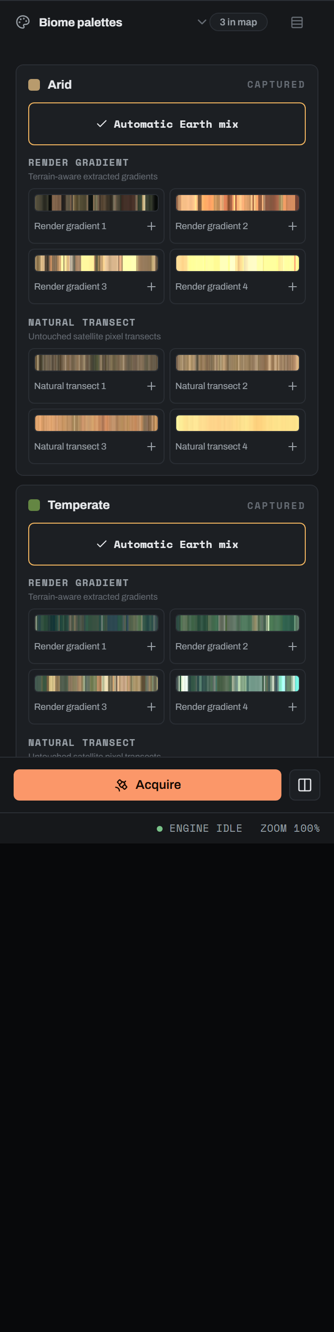
By default the engine blends a macro's variants by their Earth-share weights, which is the Automatic Earth mix card.
| Control | Engine key | Default | Range | What it does |
|---|---|---|---|---|
| Automatic Earth mix | omit the macro from palettes and palette_preferences | on for every macro | per macro | The Earth-share blend. Omitting a macro is bit-identical to the default. |
| Ordered preference list | palette_preferences | none | {macro: [ordered pv1 ids]} | An ordered multi-selection. n choices map to raw scores n down to 1, normalised to sum 1. Unselected variants are dropped. |
not exposed | palettes | none | {macro: variant_index} | A hard pick in the order returned by GET /api/worlds/{id}/palettes. Zero-weight variants drop out, so a one-hot pick collapses to a single-LUT macro. A bad pick warns and degrades to Auto rather than failing. |
palettes and palette_preferences cannot be combined; sending both is an error. Preference ids are opaque pv1:<macro>:<sha256> values bound to exact package PNG bytes, and they resolve only against the immutable captured catalogue. Unknown, duplicate, cross-biome and stale ids all fail closed with a 422, and rendering and export are blocked while the catalogue is in error rather than quietly substituting a different look. Project overrides deliberately do not participate in the captured catalogue, because they have no pinned provenance.
Cards are named by climate rather than by region, because the variant metadata carries no region or tile provenance. You get "Hot desert", never "Sahara". The two families in the panel are Render gradient (terrain-aware extracted gradients) and Natural transect (untouched satellite pixel transects).
Lithology provinces#
The variant a pixel actually gets is chosen by a shared lithology field, so a geological province continues across a climate border. Variants cross-fade continuously: the field is ranked to its land-area distribution, each variant is pure only at the centre of its Earth-share band, and a pixel lerps the two variants bracketing it. The old hard threshold read as a camouflage patchwork.
| Control | Engine key | Default | Range | What it does |
|---|---|---|---|---|
not exposed | lith_sigma_km | 160.0 km | wire 0 to 2000 km | Province scale. Four-octave noise at persistence 0.35, so outlines are rugged rather than oval blobs. In the defaults response but with no slider. |
not exposed | lith_relief | 0.85 | not bounds-checked | Couples the field to smoothed elevation. Since variants are brightness-ordered, uplands lean dark (exposed rock massifs) and basins collect bright material (sand seas). |
not exposed | lith_soften | 0.4 | wire 0 to 1 | Pulls every variant toward its macro's weighted-mean tone, so provinces read as shifts inside one material family. In the defaults response but with no slider. |
not exposed | lith_flow | 0.6 | not bounds-checked | Pushes the field toward the bright, alluvial end along routed flow, giving sediment ribbons across dark provinces. Inert without rivers. |
The variant budget#
A small crop realistically sits inside one or two material provinces, so the number of variants that survive per macro is 1 + int(extent / lith_sigma_km / 2), using the geometric-mean extent. Which ones survive is a weighted, seed-deterministic draw that does not depend on the order macros are evaluated in.
The practical consequence: a 200 km section at the default 160 km province scale gets exactly one variant per macro, no matter how many the palette bank holds and no matter how many you selected in the panel. You will see your top preference and nothing else. Raise the extent or lower lith_sigma_km if you need the spread.
Relief and hillshade#
Two knobs, and they are not interchangeable. Relief changes the pattern of the shading, meaning how steep the terrain reads. Relief shading changes its opacity, meaning how much it darkens.
| Control | Engine key | Default | Range | What it does |
|---|---|---|---|---|
| Relief | hillshade_exag (top-level render field) | 3.0× | 0.5 to 6×, step 0.1 | Vertical exaggeration of the hillshade. |
| Relief shading | hillshade_strength | 100 % | 0 to 100 %, step 5 | Lerps the shade multiplier toward unity. At exactly 100 % the output is byte-identical to the historical shade. At 0 % the hillshade pass is skipped outright. |
not exposed | hs_lo | 0.55 | not bounds-checked | Ambient floor of shade = hs_lo + hs_hi × hs. |
not exposed | hs_hi | 0.75 | not bounds-checked | Lit gain of the same expression. |
not exposed | sun_az_deg | 315.0° | not bounds-checked | Key-light azimuth. |
not exposed | sun_alt_deg | 45.0° | not bounds-checked | Key-light altitude. |
Exaggeration zero is not shading off#
This is the documented trap. Zero exaggeration collapses the gradient, so hs becomes a uniform sin(45°) = 0.7071 and shade = 0.55 + 0.75 × 0.7071 = 1.0803 for every land pixel. Every one of them is multiplied by 1.08 and then clipped, so anything already above 0.926 (snow, ice, sand, pale sediment) blows out to flat white. That is an over-exposed image. The slider floors at 0.5 but the API allows 0.
To take shading off, set Relief shading to 0 %. That skips the pass entirely, which is also a real memory and time saving: the hillshade holds around seven full native float32 planes of transient, measured at +367 MB at 4096 px native, +1549 MB at 8192, and about 6.2 GB at 16K, costing roughly 5 seconds there.
At 0 % strength the shallow-seabed ghost renders visible but unlit, which is the same decision the albedo export layer takes.
Native anchoring#
Real terrain is self-affine, so finer sampling genuinely measures steeper slopes. Measured slope goes as pitch to the power -0.61 in the Himalaya and -0.51 in the Andes, and hillshade contrast changed by a factor of about 2.6 from a 512 px preview to native before this was fixed.
The exaggeration now compensates by (working pitch / native pitch)^0.55. It is identity at native, so finished renders are bit-stable and only previews move toward them. The same compensation applies to the atlas, spectral and hypsometric styles. In equirect globe mode a per-row cosine of latitude correction is applied to east-west slopes and to the hillshade.
hillshade_strength is recorded in the render parameter metadata, so changing it invalidates a cached render exactly like a sea or snow change does.
The albedo layer#
satellite_albedo is the same composite minus the hillshade multiply and minus the seabed ghost's lighting, which is the albedo a DCC application wants. It is emitted from the same traversal as the colour, so it costs roughly 5 to 10 % extra rather than the 100 % a second render would. Requested on its own it is a full render. Requested alongside a satellite layer it reuses that render's unlit plane and completes almost instantly. It is section-only.
Colour grade and post-process#
There is no global colour grade in Dayside. No hue, mood, contrast or temperature control exists in the engine, the server or the panel. Grade the exported image in your compositor, and use the albedo layer if you want to relight rather than regrade.
What the Global look group actually holds is two cost and determinism controls alongside the two relief sliders.
| Control | Engine key | Default | Range | What it does |
|---|---|---|---|---|
| Texture detail | analysis_long_side (top-level render field) | 4096 px | 1024 to 8192 px, step 512 | Long side of the analysis grid. A speed and quality trade. It is not an output size. Labels itself Draft at or below 2048, Balanced at or below 4096, Fine at or below 6144, Maximum above. |
| Seed | seed (top-level render field) | the section's provenance seed, else 7 | any integer | Re-rolls the procedural fields. |
not exposed | style (top-level render field) | satellite | satellite, atlas, spectral, hypsometric | The colour style. Only satellite reads any parameter on this page. |
Texture detail used to swing river width by a factor of eight. Since the invariance work it does what its name says and nothing else. Drop to Draft while you dial in climate, snow and lakes, then put it back for the version you keep.
Seed re-rolls the mid-frequency mottling, the lithology provinces, the variant budget draw and the ecotone dither. Terrain and climate are untouched. Every procedural field draws from its own child generator, so adding an octave in one subsystem never re-phases another field's geography.
What does run after the colour#
Enhance section colour is the one post-process that exists. It adds learned high-frequency detail to luminance; hue and water stay analytic. It needs a persisted native-resolution analytic render first, it runs on the GPU, and its result is fresh only while the analytic base it consumed is still on disk and still hashes the same. See Enhancing terrain and the enhance section of Rendering the satellite image.
The export layers satellite_albedo and water_mask are the two outputs designed for downstream work rather than for viewing. Both are section-only and both ride the same composite traversal as the colour.
Silent caps in one place#
These are the places where what you set is not what runs. Where the interface tells you, this says how.
- Transition width is capped at about 10 % of the section extent. The exact clamp is
min(koppen_blur_km, 0.1 × √(grid area) × pitch), and grid times pitch is the extent, so it is 10 % of the geometric-mean extent in km. The server publishes it askoppen_blur_cap_km, and the slider shows an amberCAPPED AT n KM ON THIS MAPnote. Above the cap the slider does nothing at all. The cap is published only when the world records an extent; without one the server sends null, the note never appears, and the engine still clamps from the analysis grid. - The Köppen source pitch can raise the blur above your setting. The blur is first raised to at least 1.5 source cells, then the extent cap applies. A focus crop taken from a coarse world raster gets a wider ecotone than the slider says, on purpose, to melt the source's nearest-neighbour staircase. Nothing in the interface reports this.
- The climate blur is a separate, tighter number. Temperature and the authored-ice cap use
min(max(1.5 × source pitch, 3.0 km), transition width). Precipitation uses the wide transition width. Do not describe or tune them as one dial. - River width caps at 12 km and floors at one output pixel with alpha equal to width over pitch. Neither end is a tuning knob.
- River channels are gated out of depression fills. Cells with fill depth at or above 6 m by default never seed channel geometry, and the wetness term reverts to the terrain proxy there.
- Any km parameter finer than the working pitch cannot be drawn. Conversion floors at 1 px. The default 1.0 km beach ring is 0.51 px wide on a 1000 km section at a 512 px grid and simply fades out. This is expected behaviour.
- Blurs wider than 48 px decimate, blur and upsample. This is visually identical, since the fields are band-limited below the cutoff, and it bounds a cost that is otherwise linear in sigma.
- The variant budget collapses a macro's palette on a small section. A 200 km section at the default province scale shows one variant per macro. Your other preferences are simply not drawn.
- Six controls are inert without rivers, and the panel greys them out: Flow widening, Green banks, River strength, Lakes, Dryness and Min size. So are Drainage greening with its Reverse, and the unexposed
base_flowandlith_flow. - Coast blend does not move river colour. River tint is always blurred at the default 25 km whatever you set.
- Lakes are off by default, and they change the paint only. Turning them on solves standing water in the depressions the routing already measured; it does not re-route flow or move rivers. Enclosed pockets route as land whether or not you use the toggle.
- Relief at 0 is not shading off. It over-exposes. Use Relief shading at 0 %.
- The globe pass has no rivers and no lakes, because it routes no flow, and its class-weight blur does not wrap the dateline. The equirect pass also applies its own parameter overrides before yours: a 150 km transition width, a 350 km geology wavelength, a 560 km province scale, wider moisture and cavity windows, a 60 km chaos wavelength and a 45 km dither patch size. Section defaults are km-scale and would fall below one pixel at a globe's roughly 10 km/px pitch, turning climate borders into hard poster edges.
- A world with no Köppen layer reads everything at or above 18 °C as tropical, so 2000 mm/yr, which is very wet for both the snow and lake models. Arid and mediterranean climates cannot be placed at all.
- Enhance never substitutes on export. The
satellite_enhancedlayer refuses with a 422 rather than shipping the analytic image under the enhanced name.
extent_km is reachable from the current onboarding paths. On one, the server sends koppen_blur_cap_km: null, so Transition width caps silently with no note.Legacy keys, do not tune#
These are still accepted, still in the defaults response, or still in the code. None of them steers the current render. Tuning them wastes your time.
| Key or behaviour | Status | What replaced it |
|---|---|---|
river_t0 (0.08) and river_t1 (0.38) | Legacy. Still on the wire, still bounds-checked, no slider anywhere. | river_min_catchment_km2 and river_width_km. The old smoothstep window only runs when a caller passes no catchment field, which means direct engine calls and old tooling. The server render path has ignored them since the invariance work. |
| The percentile river transfer | Legacy path only | The absolute catchment threshold. |
river_dark (0.30) | Renamed | river_blend (0.55), a blend strength rather than a darkening depth. |
| The dark-only river multiply | Removed | Climate-keyed river tint per macro. |
| Snow as a smoothstep on mean annual temperature | Removed | The mass-balance model: summer temperature against accumulation at the equilibrium line. |
t_snow_c as a threshold | Re-meaning, same slider, same direction | A bias on the Ohmura critical temperature, neutral at -2.0 °C. |
| Every cell at or below 0 m is sea | Superseded whenever the flow routing runs, lakes on or off | Border-connected water plus authored-canvas ocean. Everything else below 0 m is an enclosed pocket that routes as land. |
ocean.png and its 6500 m depth constant | Legacy, still loaded, never sampled | The four-zone sea optical model. |
| Single-LUT-per-macro gradient loading | Legacy | Variant sets with Earth-share weights. |
| The fractal domain warp | Removed, and it is a standing directive not to reintroduce it | Authored Köppen shapes plus the physical fields. |
ecotone_dither at 0.65 | Caused the camouflage regression | Default 0.0, hard maximum 0.15. |
koppen_blur_km at 80 km | Retuned | 25 km, a boundary that is defined but soft. |
analysis_long_side as a look control | It used to swing river width eightfold | A pure speed and detail trade, as the name promises. |
river_mask, snow_mask, normal_map export layers | Deferred, greyed in the export modal | water_mask ships as the recomputable superset of river_mask. The other two have no writers. |